Last updated 12 Feb 2004. Questions and feedback welcome.

The Proteome Browser provides a wealth of protein information presented in the form of graphical images and links to external internet sites.

UniProtKB information: The top line of the page shows the UniProtKB accession number, entry name, and protein name for the current selection. Click on the accession number to open the record for this protein in the UniProtKB database.

Proteome browser tracks: The tracks image displays a set of aligned tracks showing information about the protein's amino acid sequence and anomalies, the corresponding DNA sequence and exon make-up, and protein traits such as hydrophobicity, glycosylation potential, polarity, cysteine content, and SuperFamily domain composition. To display a description of a track from the Protein Browser web page, click on the track's label. For more information about the individual tracks, see the Protein Tracks section.

The navigation buttons permit scrolling and resizing of the tracks image:

• Scrolling left or right: To shift the browser tracks image sideways to the left or right by 2%, 47.5%, or 95% of the displayed size, click the corresponding move arrow.
• Rescaling the image: The Rescale to buttons control the size of the tracks image. At the default "Full" setting, the image is displayed at its full size. The "1/2" and "1/6" buttons shrink the image size by the equivalent amount. The image retains its scrolled settings when it is rescaled. The amino acid sequence of the protein is displayed only in the full-sized image.
• Displaying the Genomic sequence: To view the codons that correspond to the Amino Acid Sequence track and their reverse complements, click the DNA rescale button. The Genomic Sequence track is hidden by default.

Protein property histograms: The Protein Browser's histogram section provides a graphical comparison of several protein traits relative to those of proteins genome-wide. The pictured traits include amino acid frequencies and anomalies, molecular weight, exon count, cysteine abundance, hydrophobicity, isoelectric point, and predicted domains. To display a brief description of a histogram from the Protein Browser web page, click on the graph's label. For detailed information on the histograms, see the Protein Property Histograms section.

UCSC links: These links display additional information about the gene and mRNA associated with the selected protein.

• Genome Browser link: Click on the accession number to open up a Genome Browser window displaying this mRNA.
• Gene Details Page link: Click on the accession number to display the Genome Browser Known Genes details page for the gene associated with this protein.
• Gene Sorter link: Click on the accession number to open up a Gene Sorter window displaying the gene associated with this mRNA, along with a set of related genes.

Domain information: The browser provides 3 primary sources of detailed domain information about the selected protein.

• SuperFamily/SCOP track: See the Protein Tracks section for a description of this track. Click on a yellow domain box in the track to display Superfamily information about that domain.
• EMBL-EBI InterPro website link: Click on the Graphical view of domain structure link to open a page showing protein matches from the UniProtKB database. Click on an ID number to display the InterPro information page for that domain.
• Sanger Institute Pfam (Protein families database of alignments and HMMs) website link: Click on the Pfam accession number to display the Pfam database record for the domain.

Comparative 3-D structures:

• Protein Data Bank (PDB): When available, this section displays one or more 3-D structures of the protein from the PDB. Click on a structure number to display the associated PDB record.
• ModBase: This section displays front, top, and Side views of the predicted comparative 3-D structure of the protein obtained from UCSF's ModBase. Click on the protein accession number or one of the images to display the ModBase database record for the protein. If no images are displayed, no ModBase structure exists for the protein.

Pathways:

• BioCarta: Provides information about gene interactions within pathways for human cellular processes, displayed on NCI's Cancer Genome Anatomy Project (CGAP) website.
• KEGG: Displays the associated pathway record in the Kyoto Encyclopedia of Genes and Genomes (KEGG).

Fasta format: This section shows the Fasta record for the protein containing the complete amino acid sequence.

This section contains a brief description of the tracks available in the Protein Browser. To view this information directly from the Proteome Browser, click the label of the track in which you are interested.

Amino Acid Scale: The top and bottom tracks provide a scale to determine the amino acid length of the selected protein. The label of the final tick mark on the scale shows the protein's total amino acid count.

NOTE: Some web browsers may not display the largest proteins correctly due to width limitations. In this case, use the arrow controls to view the carboxy end of the protein.

Amino Acid Sequence: This track shows the amino acid sequence comprising the protein. The data were obtained from the UniProtKB and TrEMBL databases.

Genomic Sequence and Complement: The display of this track varies, depending on which genomic strand the mRNA aligns to.

If the mRNA matches the forward (+) strand of the genomic sequence as displayed in the Genome Browser, the DNA sequence is displayed as a single row of nucleotides -- labeled "Genomic Sequence" -- whose codons are read directly into the amino acid sequence.

If the mRNA matches the reverse (-) strand of the genomic sequence, the track shows both strands of the DNA. The upper strand -- labeled "Coding Sequence" -- matches the mRNA, to follow the convention that a protein sequence is displayed in the amino-to-carboxy direction. The genomic sequence as displayed in the Genome Browser, therefore, is read from the lower strand (labeled "Genomic Sequence") in the reverse direction.

For example, the first few codons of the gene for human thymidylate kinase, CDC8, appear on the negative strand of chromosome 2 in the hg16 Genome Browser as:

chr2:242946915-242946940

Genomic    5'-  GAG AGC CCC GCG CCG GGC CGC CAT -3' (genomic)

Protein          M   A   A   R   R   G   A   L 
DNA        5'-  ATG GCG GCC CGG CGC GGG GCT CTC -3' (reverse complement of genomic)
Complement 3'-  TAC CGC CGG GCC GCG CCC CGA GAG -5' (reverse of the genomic)

The genomic sequence and complement displayed in this track are derived from the kgProtMap table (an alignment between protein, mRNA, and genome) and the base genome.

NOTE: This track displays only when the current scale is set to the "DNA scale" option.

Genome Browser: The heavy black line in this track shows the portion of the gene that was displayed in the window on the last Genome Browser view. If the entire gene was displayed in the browser, the line is not shown. The label above the leftmost portion of this track shows the Genome Browser coordinates corresponding to this view. Click on the line to open the UCSC Genome Browser to this position.

Exons: This track shows the position and layout of exons within the gene and their correspondence to the protein's amino acid sequence. Exons are depicted by alternating blue and green bands, and are labeled by their order number within the gene. This blue/green coloring is repeated in the DNA Sequence track, which also shows the coding phase. In cases where exon boundaries are stair-stepped, the amino acid coding has been split across two exons.

Click on an exon to display the corresponding region in the UCSC Genome Browser. See the Number of Exons histogram to view the exon count for this gene and compare it to a genome-wide statistical distribution.

The exon positions displayed in this track were derived from the kgProtMap table (an alignment of protein, mRNA, and genome data). For an in-depth discussion of the information displayed in this track, see the Exon Count section.

Polarity: This track shows the polarity of each amino acid in the protein sequence. Amino acids tending toward negative charge are represented by red blocks below the center line; amino acids tending to positive charge are represented in blue above the line. The height of the block gives some indication of relative polarity for un-ionized amino acids. For example, serine is given a lower height than aspartic acid.

The pI histogram in the Polarity discussion section shows the genome-wide statistical distribution of pI of human proteins from UniProtKB and TrEMBL. For reasons of solubility, few proteins have a pI near intra-cellular pH, resulting in a bimodal peak about this pH.

See the pI histogram to view the pI of the selected protein relative to a genome-wide statistical distribution of pI of all proteins from UniProtKB and TrEMBL. For an in-depth discussion of the information displayed in this track, see the Polarity and Isoelectric Point section.

Hydrophobicity: This track shows the distribution of hydrophobic residues across the selected protein, according to the Kyte-Doolittle scale. Using a sliding 6-amino-acid window, this scale assigns positive values to hydrophobic amino acids, which are shown in blue above the center line on the track. Hydrophilic amino acids are displayed in red below the center line.

Hydrophobic residues occur most notably in the interior of globular proteins, as trans-membrane segments, in membrane-inserted tails, or as surface patches in domains that bind to other subunits of oligomers. Hydrophilic amino acids are typically found on protein surfaces exposed to an aqueous environment.

See the Hydrophobicity histogram to view the mean hydrophobicity of this protein relative to a genome-wide distribution. For an in-depth discussion of the information displayed in this track, see the Hydrophobicity section.

Cysteines: This track shows the location of cysteines as blue blocks along the peptide chain.

Refer to the Number of Cysteines histogram to compare this protein's cysteine count to a genome-wide statistical distribution of cysteine abundance in all proteins found in this assembly. For an in-depth discussion of the information displayed in this track, see the Cysteine Count section.

Glycosylation: This track shows predicted glycosylation sites within the protein, represented by red blocks displayed below the center line. For an in-depth discussion of the information displayed in this track, see the Glycosylation section.

Superfamily/SCOP: This track shows the positions and names of predicted domains within the protein as determined by Hidden Markov Modeling (HMM) comparison to all known 3-D structures. Each predicted domain is represented by a yellow box. Click on a domain to display information about that domain on the Superfamily website. SuperFamily in turn relies on the Structural Classification of Proteins System (SCOP). This method has an advantage over Blast or psi-Blast in that protein folds are often conserved long after primary sequence alignment has become unreliable (10-25% identity range).

InterPro domains, based on clustering of sequence alignments, do not require a 3-D reference sequence and therefore complement SuperFamily domains. Refer to the InterPro Domains histogram to view the total number of predicted domains within a protein and compare this count to the number of multiple-domain proteins genome-wide. For an in-depth discussion of the information displayed in this track, see the Protein Domains section.

Amino Acid Anomalies: This track displays amino acids within the protein sequence that differ significantly in abundance from their average occurrence genome-wide. Amino acids present in excess or deficiency are denoted by red blocks above or below the center line, respectively.

See the Amino Acid Anomalies histogram to view amino acid abundances in this assembly. For an in-depth discussion of the information displayed in this track, see the Amino Acid Anomalies section.

This section contains a brief description of the histograms available in the Protein Browser. To view this information directly from the Proteome Browser, click the label of the histogram in which you are interested.

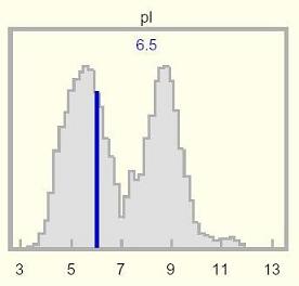
pI: The pI (isoelectric point) histogram shows the pI of the selected protein relative to a genome-wide statistical distribution of pI of all proteins from UniProtKB. TrEMBL-NEW proteins are not included in the distribution. The calculated pI of the protein is displayed at the top of the histogram, and is shown as a vertical dark blue line overlying the statistical distribution.

The distribution data were generated by using the UniProtKB pI calculation tool on the set of protein IDs.

To view the polarity of each of the amino acids in the protein sequence, see the Polarity track. For an in-depth discussion of the information displayed in this track, see the Polarity and Isoelectric Point section.

Molecular Weight: This histogram shows the selected protein's molecular weight relatve to a genome-wide statistical distribution of molecular weights of all proteins from UniProtKB. TrEMBL-NEW proteins are not included in the distribution. The molecular weight is shown at the top of the histogram, and a vertical dark blue bar indicates the weight relative to the genome-wide distribution.

The distribution data were generated by using the UniProtKB molecular weight calculation tool on the set of protein IDs. For an in-depth discussion of the information displayed in this track, see the Molecular Weight section.

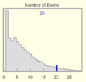
Number of Exons: This histogram displays a genome-wide statistical distribution based on the number of coding exons in the kgProtMap table. The number of coding exons in the selected protein is displayed at the top of the graph, and a dark blue vertical line highlights this count relative to the genome-wide distribution.

To view a linear depiction of the position and layout of the exons within the gene and their correspondence to the protein's amino acid sequence, see the Exons track.

The exon positions displayed in this track were derived from the kgProtMap table (an alignment of protein, mRNA, and genome data). For an in-depth discussion of the information displayed in this track, see the Exon Count section.

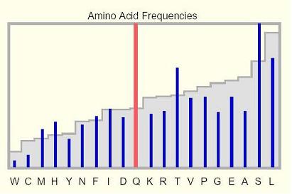
Amino Acid Frequencies: This histogram shows the abundance of amino acids within the selected protein relative to their average occurrence genome-wide. The bars of the graph indicate the genome-wide average frequencies of the amino acids, and the blue vertical lines indicate the abundance of the amino acids within the selected protein. Any amino acid with an abundance that falls outside the 2.5% to 97.5% genome-wide distribution range is represented by a red line. Genome-wide averages are based on the following Genome Browser tables from this assembly: pbAaDist[AA], pbAnomLimit, and pbResAvgStd. The amino acid data in these tables were obtained from proteins in the knownGene table that were found in UniProtKB (TrEMBL-NEW excluded). Standard deviations were derived from compositions of the genome-wide set of proteins.

See the Amino Acid Anomalies track to view specific occurrences of excessive or deficient amino acids within the protein sequence. For an in-depth discussion of the information displayed in this track, see the Amino Acid Anomalies section.

InterPro Domains: This histogram shows the number of predicted InterPro domains contained in the selected protein relative to the number of domains found in proteins genome-wide. The number of domains is shown at the top of the histogram, and is plotted on the genome-wide distribution as a vertical dark blue line. For an in-depth discussion of the information displayed in this track, see the Protein Domains section.

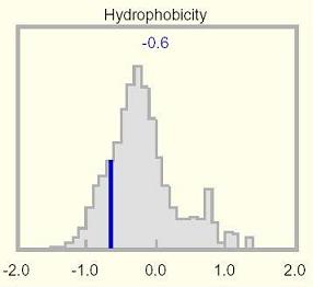
Hydrophobicity: This histogram shows the mean hydrophobicity for the selected protein relative to a genome-wide distribution of all proteins in the UniProtKB database, which is essentially a broad Gaussian centered on zero. A few proteins fall outside the plotting display range and are not accounted for in this distribution. The mean hydrophobicity is shown at the top of the histogram, and is indicated by a dark blue vertical line overlying the genome-wide distribution.

To view the distribution of hydrophobic residues across the selected protein, see the Hydrophobicity track. For an in-depth discussion of the information displayed in this track, see the Hydrophobicity section.

Number of Cysteines: This histogram compares the selected protein's cysteine count to a genome-wide statistical distribution of cysteine abundance in human proteins, based on the cysteine abundance in all proteins found in the Known Genes data set for this genome assembly. The number of cysteines in this protein is shown at the top of the graph, and its relative position in the genome is indicated by a dark blue vertical line overlying the genome-wide distribution histogram.

To view the locations of cysteines along the peptide chain, see the Cysteines track. For an in-depth discussion of the information displayed in this track, see the Cysteine Count section.

Amino Acid Anomalies: This histogram displays the extent to which certain amino acids within the protein sequence differ in abundance from their average occurrence genome-wide. Amino acids present in excessive or deficient amounts are represented by a red vertical bar extending above or below the middle line, respectively. The height of the bar indicates the degree of departure of the amino acid frequency from the expected value genome-wide.

The histogram is based on the following Genome Browser tables from this assembly: pbAaDist[AA], pbAnomLimit, and pbResAvgStd. The amino acid data in these tables were obtained from UniProtKB. Amino acids are flagged as anomalous if their occurrence in a protein falls outside the 2.5% to 97.5% genome-wide distribution range. Proteins with fewer than 100 amino acids have been filtered from the sample to exclude variances attributable to short length.

See the Amino Acid Frequencies histogram to view amino acid abundances in this assembly. For an in-depth discussion of the information displayed in this track, see the Amino Acid Anomalies section.

Within an orthologous gene family, the exon number, exon locations, length, and coding phase (how a codon is split between consecutive exons) are usually conserved from mammal to fugu, but not to nematode or fruit fly. Paralogous gene families do not necessarily conserve any of these attributes when gene duplications are very old, as is the case with the 17 members of the mammalian sulfatase family.

The genome-wide statistical distribution is based on protein data from the kgProtMap table (an alignment of protein, mRNA, and genome data). These data are somewhat distorted because a small number of alternatively spliced genes are counted more than once, and the first and last exons of many predicted genes are incomplete.

Long introns give rise to systematic errors in the tables, because predicted genes are often unwittingly split into two or more pieces. This skews the exon number distribution toward lower counts. In some cases, purely UTR exons are inappropriately included. While further work will improve and add many gene models, the overall affect on statistics may be slight.

Reference mRNAs do not always align fully anywhere in the genome for a variety of reasons as determined by Blat. It is worth distinguishing gaps in the genomic sequence that may disappear in later assemblies and indel polymorphisms in the mRNA relative to the genome. For example, genomic PRNP is 24 bp shorter than 98% of mRNAs from random subjects. Blat is not reliably capable of finding short exons in long introns, the shortest known being a two-codon exon. These latter problems do not go away with finished genome, although many short exons could be successfully force-fit by a second, tuned Blat pass, given the constrained target intron and phase consistency requirements.

On the Proteome Browser display, the amino acid sequence is derived from its experimental evidence, the mRNA, whereas the exon track comes from the genomic alignment. When a piece of the mRNA cannot be aligned, it is grayed out and not assigned an exon number. This results in unstable exon numbers downstream, and perhaps gives unfamiliar numbers to well-known exons in certain genes assigned in the experimental literature. However, exon numbering is dynamic, as new 5' UTR exons are often found over time. Numbering exons from the start codon is vulnerable to alternative translation starts. With alternative splicing, there may not be a consistently dominant or naturally canonical form in all tissues to initiate numbering. Thus, there is no consensus on exon numbering at this time.

The information presented in the Exons track can be verified and adjusted by comparing it with the Gap track in the Genome Browser. If an unalignable piece commences at a gap but re-commences later after good genomic sequence, the Proteome Browser may treat it as an extension of the proximal exon but display it in gray to indicate uncertainty through the other cases. Also, if the mRNA coding has an insertion relative to the base genomic sequence, it is indicated by a gray bar in the Exon display.

It is advisable to place some sort of cutoff on mRNA-derived protein length. Proteins under 100 amino acids are often fragments, mispredictions, or simply artifacts. To set the cut-off objectively, the length distribution plot was sampled for hand-curation at the low end (5 putative proteins in each block-of-ten range, e.g., 30 - 40 amino acids) to examine the evidence. The quality increases monotonically with greater length; the cutoff was set at 80% or greater having meaningful other supporting documentation.

Exon count in mammals has an early peak that declines rapidly and monotonically to a very long tail reaching out to 363 exons (which code for 38,138 amino acids) in the human gene titin. The KIAA cDNA Human Unidentified Gene-Encoded database (HUGE) has somewhat corrected for a very significant experimental and annotation bias against long proteins.

Genes with a single coding exon appear in excess, but this is distorted by certain large gene families (olfactory receptors), gene fragments, and unrecognized processed pseudogenes. Human ribosomal proteins alone have over 2000 known pseudogenes). Discounting this, a single peak would occur at 4 exons (7.4% of all genes). There remains a substantial annotation bias toward fewer exons as prediction software tends to split genes possessing long introns -- the number of genes in the Ensembl human gene collection declined by nearly 7500 genes to 21,787 in progressing to NCBI assembly 34 (UCSC version hg16).

Proteins are charged due to amino acid side chains, secondary modifications, and unblocked terminal residues. The net charge swings from negative to positive according to the pH of the ambient water and the local environment of each contributing residue in the folded protein. The pI is the pH that results in a net charge of zero.

The pI is a useful property because it predicts solubility properties and so suggests the cellular environment in which a protein will be found. By displaying an individual protein's pI over the histogram of genome-wide pI distribution, the Protein Browser calls attention to unusual values of pI that could be clues to function or location. For example, human pepsin A has a pI of 3.4, consistent with its expression in the highly acidic stomach; human cytochrome c has a pI of 9.6 appropriate to binding negatively-charged membrane phospholipid. At the isoelectric-focusing stage of 2-D electrophoresis, each protein migrates to its isoelectric point. A protein migrating anomalously may have an unsuspected covalent modification.

The pI algorithm uses pK values for relevant amino acids (C, D, E, H, K, R, S, T, Y, and amino- and carboxy- termini) derived experimentally for model peptides in 9 M urea at 25 degrees C. The prediction tool removes predicted signal peptides, but does not consider other modifications. It is least accurate on small proteins with limited intrinsic buffering capacity, with highly basic proteins where pI lacks a solid experimental foundation, and on protein domains buried in membrane. Raw sequence is used when no UniProtKB accession is available.

Clearly, it is not feasible to precisely predict pI for native proteins because this requires knowledge of how the local folded environment has affected ionization propensities (pK) of individual contributing residues. A notable example is histidine, the residue most sensitive to slight variations around neutral pH. Furthermore, biologically relevant pI is a property of mature proteins but not all processing steps can be reliably predicted. Modification may cycle on and off in vivo according to regulatory status -- for example, many proteins are transiently phosphorylated.

Genome-wide experimental determination of the pI of native proteins cannot be accomplished on a microarray because each protein would have to be correctly processed, folded, and modified. Some relevant modifications, such as sialylated glycosylation, are not yet achievable in vitro and can vary by cell type. Nonetheless, the predicted pI values are accurate enough for many purposes.

It is likely that intrinsic membrane proteins are under-represented in the data set because they are more difficult to purify than peripheral or cytosolic proteins. The mammalian pI distribution seems adequately modeled by an acidic Gaussian centered on pH 5.8, a pronounced trough at pH 7.4, and an alkaline Gaussian centered on pH 8.8. The near-neutral pI region has presumably been depleted by selective pressure -- cytoplasmic proteins are least soluble at their isoelectric point. Proteins may be evolutionarily trapped on one side of the valley or the other.

The molecular weight of a protein in kilodaltons (kD) can be estimated by adding 10% to its length in amino acids, then dividing by 10. For example, a 400-residue protein is approximately 44 kD, based on an average of 110 daltons per amino acid, assuming random composition.

More accurately, as is done in the Protein Browser, a protein's weight can be calculated from the individual molecular weights of the amino acids. Processed signal peptides and covalent modifications (possibly transient or partial) must be taken into account, depending on the situation.

The molecular weights displayed in the Protein Browser have been taken from UniProtKB when accession numbers were available; otherwise, they have been based on genomic sequence as processed with the UniProtKB molecular weight tool. This reflects the removal of isotopic abundances and predicted signal peptides, but not modified amino acids. Numbers have been rounded to the nearest kD, which suffices for gel migration (although clearly not for mass spectroscopy). For genomics purposes, the amino acid count of a full-length coded protein is more useful than its molecular weight.

It is likely that intrinsic membrane proteins and very long proteins are under-represented in this data set. The display thus calls attention to unusual molecular weight values that could suggest multiple domains or chain fusion, which can be lineage-specific events. On predicted protein tracks, molecular weights below 100 kD may indicate an incompletely-predicted protein.

Mammalian molecular weights average 56 kD (627 aa) in the data set used. The distribution exhibits a very long tail of a few proteins with much higher molecular weights. Larger proteins are under-represented in genomic predicted tracks because of incomplete cDNAs and long introns. Conversely, short proteins may be merged or missed altogether. At present, mammalian proteins appear to be somewhat smaller than the average Drosophila protein (649 aa), but approximately 80% larger than the average E. coli protein (350 aa). Larger size suggests increased domain content. Because 120 kD can suffice to encode a stand-alone functioning enzyme (e.g. lysozyme), 3-5 domains should be expected for the average mammalian protein.

In conjunction with other tracks and specialized prediction tools, patterns of hydrophobic residues can sometimes be interpreted structurally. Smoothing the track over a rolling window size of 6 is effective in locating surface-exposed (polar) regions, whereas a window size of 20 is better suited for defining transmembrane domains that peak at a local average hydrophobicity score of 1.6 or more. Interior hydrophobic residues, while often packed tightly and critical to protein folding and stability, may be dispersed along the linear sequence. UniProtKB offers 22 other choices of hydrophobicity scales and considerable control over smoothing the convolutions.

Using the genome-wide amino acid composition of human proteins, the averaged amino acid has a hydrophobicity close to zero (-0.018). This reflects the design of the scale, the need for surface polar and charged residues to maintain solubility, and the frequencies of cytoplasmic and membrane-bound proteins. The track uses a baseline of zero.

The mean hydrophobicity of the selected protein illustrated in the Hydrophobicity histogram is not always informative, because transmembrane domains can be offset by highly polar regions elsewhere, yielding an overall mundane value. Unusual values may be apparent in the Hydrophobicity track, and will also surface as amino acid compositional anomalies.

Kyte-Doolittle hydrophobicity scale

J. Mol. Biol. 157:105-132(1982) Ile: +4.5 Val: +4.2 Leu: +3.8 Phe: +2.8 Cys: +2.5 Met: +1.9 Ala: +1.8 Gly: -0.4 Thr: -0.7 Ser: -0.8 Trp: -0.9 Tyr: -1.3 Pro: -1.6 His: -3.2 Asn: -3.5 Asp: -3.5 Gln: -3.5 Glu: -3.5 Lys: -3.9 Arg: -4.5

Cysteine is not a common amino acid, with an abundance of 2.3% genome-wide, being most often found paired in disulfides. Disulfides in human proteins are found almost exclusively in oxidative environments, such as on the cell surface or in lysosomes, but not in the cytoplasm or the nucleus. Therefore, high cysteine content, after discounting for iron-sulfur cluster proteins, is contra-indicative of a cytoplasmic location. Similarly, the presence of glycosylation sites, as cell-surface indicators, suggests that cysteines in a protein will usually be paired.

The Cysteines track shows where cysteines occur along the peptide chain, but does not predict whether a given cysteine occurs in a disulfide or where its partner is located. The two cysteines linked in a disulfide are not necessarily located near one another in the amino acid sequence or even in the same chain. Rather, the correct cysteine residues are brought into proximity during protein folding, which may bring remote cysteine residues together. Mammals have an extensive disulfide isomerase activity in the endoplasmic reticulum believed to chaperon disulfides toward the correct pairing (and thus correct folding).

Cystine-pair information is available when the 3-D structure is known, when the selected protein can be threaded to a known structure, when a satisfactory ab initio model exists, or by sequence alignment homology. UniProtKB has also collected experimentally-determined disulfides from the literature.

Various web tools can predict disulfide bonds with varying degrees of success [1-4]. Intermolecular disulfides are fairly common, yet the partners often unknown and so very difficult to take into account. Where reliably predictable, disulfides provide a strong geometrical constraint on ab initio structure prediction to applicable proteins.

Disulfide bonds are fairly well-conserved evolutionarily in many protein families, even as the percent identity drops below 35%. However, in some deeply diverged families such as sulfatases, new disulfides have emerged in subfamily lineages and no ancient disulfides are retained. Conserved cysteines that are not part of an active site are distinguishable from sporadic cysteines and are likely in a disulfide. If the family is large enough and the number of cysteines fairly small, the pairing pattern can sometimes be inferred, starting with the two best-conserved cysteines found in the deepest alignment. Other proteins, with complex disulfide knots, are intractable to homology methods.

Certain protein domains have characteristic disulfide motifs, for example, the CxxxCxxC 4Fe­4S clusters in radical SAM enzymes. These are often preserved even as the domain finds itself in a much larger protein with many additional cysteines. The domain tool Pfam provides 28 domain listings under disulfide.

Another special case occurs in transmembrane proteins. For example, ectodomain cysteines will not be paired with transmembrane or endodomain cysteines. Being external to the cell, they are likely in disulfides although the pairing is not always resolved and indeed may be intermolecular.

Disulfide bond prediction references:

1. Fariselli P, Casadio R. Prediction of disulfide connectivity in proteins . Bioinformatics 2001 Oct;17(10):957-64.
2. Fariselli P, Riccobelli P, Casadio R. Role of evolutionary information in predicting the disulfide-bonding state of cysteine in proteins. Proteins 1999 Aug 15;36(3):340-6.
3. Martelli PL, Fariselli P, Malaguti L, Casadio R. Prediction of the disulfide bonding state of cysteines in proteins with hidden neural networks. Protein Eng. 2002 Dec;15(12):951-3.
4. Mucchielli-Giorgi MH, Hazout S, Tuffery P. Predicting the disulfide bonding state of cysteines using protein descriptors. Proteins 2002 Feb 15;46(3):243-9.

N-glycosylation sites (along with disulfides) predict the cellular location of proteins to a certain extent. Proteins are glycosylated on an internal asperagine residue as they pass through the endoplasmic reticulum for export. Glycosylation affects protein folding, trafficking, solubility, antigenicity, half-life, localization, and cell-to-cell interactions.

Potential N-glycosylation sites are reliably predicted by a tripeptide motif, NxT or NxS, where x is not proline and P seldom follows. Multiple motifs in mature regions of the same protein and conservation in homologs provide significant additional support. Glycoproteins are targeted to the cell exterior, lysosome or similar compartment, and extra-cellular space, but not to the cytoplasm, nucleus, or mitochondria. Predictions can sometimes be reinforced by the presence of a signal peptide or a glycosylphosphatidylinositol (GPI) membrane terminal anchor.

Actual occupancy of N-glycosylation sites in vivo is hard to predict. Specific sites may be substituted to varying degrees of saturation in various tissues at different developmental stages, and complex carbohydrate moieties are not always fully built-out. The three amino acids involved are very common; therefore, many chance occurrences happen, which can be estimated as occurrence of the reversed motif. Thus, the number of glycosylation sites used genome-wide can be estimated as the excess, (NxT + NxS) - (TxN + SxN), x not P. However, this does not address glycosylation of specific motifs. Some glycosylation sites are quite ancient, but others have been gained or lost over moderate time scales in paralog familes.

Conservation of a potential motif in mammals provides only weak support for its utilization. Because overall protein conservation is 85% between -- for example -- mouse and human, the 2-amino-acid motif would be invariant 72% of the time without its necessarily being conserved due to selection. Even observed conservation between pufferfish and human is not persuasive (50% chance). The motif might be conserved for catalytic or structural reasons, not glycosylation. However, a persuasive case can sometimes be made from integration of all available information on a given protein.

At present, approximately half of all human proteins have a recognizable domain using SuperFamily. However if no relevant crystallographic or NMR structure has been determined, no match will appear in this track even though a well-known domain might readily be identifiable by alignment methods. Domains of membrane proteins and difficult-to-study proteins are therefore under-represented in the track, leading to a bias in favor of the smaller soluble proteins found at the Protein Data Bank (PDB). Furthermore, some proteins have been studied as truncated, more-easily crystallized fragments and not all domains will have been detected. These biases are seen clearly in the statistical breakdown of the 1073 currently known superfamilies (all species, including 733 in human).

Superfamilies go so far back in evolutionary time that branches have sometimes evolved quite different functions despite retaining the same fold. These functions may be distinct but plausibly related, as in the alkaline phosphatase superfamily where 17 human members have become sulfatases. Or, the functions may be so diverged, as in the TIM beta/alpha-barrel family, that multiple independent evolutionary development of the same fold seems possible. Thus, functional interpretation of a match in the domain track requires a measure of caution.

For humans, the current distribution of observed domains is dominated by thousands each of zinc fingers, immunoglobulin domains, P-loop NTPases, laminins, cadherins, olfactory genes, fibronectins, and protein kinases. At the other extreme, 114 domains are known only from single protein representatives.

Some functional classes, such as extra-cellular matrix proteins, commonly have both multiple domain types and multiple copies of a given domain. Human proteins average only 1.5 currently detectable domains per protein and a large number of superfamilies have but one domain (although these are mostly in small families). Mammalian proteins are some 50% larger than the average E. coli protein (450 vs 300 amino acids) but some of this is attributable to ragged growth at poorly conserved N- and C- termini.

If the 20 amino acids were used equally, each would occur at a level of 5% in every protein (excluding selenocysteine, whose total occurrence numbers a few dozen). Of course, the amino acid composition of proteins genome-wide is actually quite different, with some residues in excess and others consistently depleted. For example, leucine has an average occurrence of 9.7%, over seven times the abundance of tryptophan at 1.3%. Furthermore, individual protein composition can differ markedly from these averages due to a variety of structural and functional reasons, such as long unstable runs of a single amino acid or the periodic residues in collagen helices. Higher ambient GC content in a patch of chromosome can also influence the amino acid content at weakly-conserved residues, in part from fixation of CpG hotspot mutations.

The Protein Browser displays two histograms showing amino acid frequencies and anomalies within the selected protein, arrayed according to abundance. These anomalies can contain useful clues to subcellular location, protein structure, function, and mutational propensity. The distribution of anomalies along the protein primary sequence is shown in the AA Anomalies track.

Compositional anomalies in general have no ready explanations. Indeed, a certain number of departures from mean composition are expected for purely statistical reasons. Anomalies may reflect a bulk physical attribute, such as the need for many charged residues, or avoided residues (cysteines stabilizing misfolding through disulfides). Anomalies may arise from internal sequence repeats, such as runs of a single amino acid, or longer-period structural repeats, with every third residue being glycine to pack the triple helix of collagen. At longer scales, multiply-repeated domains can skew overall composition. Thus, compositional anomalies suggest unusual overall amino acid abundances without necessarily suggesting an explanation.

Tables of amino acid usage are available elsewhere for other species by codon and for UniProtKB as a whole.

Amino acid abundances based on the pepResDist table (July 2003 human assembly)